1-1. Pokemon Generation One 데이터셋
* Pokemon Generation One 데이터셋은 포켓몬 시리즈의 첫 번째 세대(Generation One)에 등장하는 151마리 포켓몬의 이미지와 정보를 포함한 데이터셋입니다.
* 이 데이터셋은 주로 컴퓨터 비전과 머신러닝 작업(예: 이미지 분류, 객체 감지, 스타일 전환 등)에 활용됩니다.
* 이 데이터 세트에는 149개의 폴더가 포함되어 있으며, 각 폴더에는 각 포켓몬 1세대당 하나씩 포함되어 있으며 각 폴더에는 각 포켓몬당 60개의 이미지가 포함되어 있습니다.
* 총 10,000개 이상의 이미지가 있습니다.
링크 주소 : https://www.kaggle.com/datasets/thedagger/pokemon-generation-one/data
Pokemon Generation One
Gotta train 'em all!
www.kaggle.com
1-2. Complete Pokemon Image Dataset
* Complete Pokemon Image 데이터셋은 Kaggle에서 제공되는 데이터셋으로 모두 https://pokemondb.net/ 에서 스크랩된 것입니다.
* 포켓몬 세대 1부터 8까지의 2,500개 이상의 깨끗하게 라벨링된 이미지를 포함하고 있습니다.
* 이 데이터셋은 각 포켓몬의 다양한 형태와 자세를 포괄하며, 이미지 분류, 객체 인식, 생성 모델 등 다양한 딥러닝 및 머신러닝 작업에 유용하게 활용될 수 있습니다.
* 이미지들은 고품질로 제공되어 모델 학습 시 정확한 특징 추출에 도움이 됩니다.
링크 주소 : https://www.kaggle.com/datasets/hlrhegemony/pokemon-image-dataset
Complete Pokemon Image Dataset
2,500+ clean labeled images, all official art, for Generations 1 through 8.
www.kaggle.com
참고 링크 주소 : https://github.com/hoya012/deep_learning_object_detection
GitHub - hoya012/deep_learning_object_detection: A paper list of object detection using deep learning.
A paper list of object detection using deep learning. - hoya012/deep_learning_object_detection
github.com
예시 1)
!kaggle datasets download thedagger/pokemon-generation-one
-->
Dataset URL: https://www.kaggle.com/datasets/thedagger/pokemon-generation-one
License(s): GPL-2.0
Downloading pokemon-generation-one.zip to /content
 99% 2.13G/2.15G [00:20<00:00, 240MB/s]
100% 2.15G/2.15G [00:20<00:00, 114MB/s]
예시 2)
#압축을 품
!unzip -q /content/pokemon-generation-one.zip
예시 3)
!kaggle datasets download hlrhegemony/pokemon-image-dataset
-->
Dataset URL: https://www.kaggle.com/datasets/hlrhegemony/pokemon-image-dataset
License(s): CC0-1.0
Downloading pokemon-image-dataset.zip to /content
 97% 56.0M/57.9M [00:00<00:00, 199MB/s]
100% 57.9M/57.9M [00:00<00:00, 180MB/s]
예시 4)
# 압축을 품
!unzip -q /content/pokemon-image-dataset.zip
예시 5)
!mv dataset train
예시 6)
# train/dataset 삭제
!rm -rf train/dataset
예시 7)
# validation 이동
!mv images validation
예시 8)
import os

# 'train' 폴더 내의 모든 파일 및 디렉터리를 리스트 가져옴
train_labels = os.listdir('train')

# 가져온 라벨 리스트 출력
print(train_labels)

# 라벨(클래스)의 개수 출력
print(len(train_labels))
--->
['Golem', 'Machoke', 'Gengar', 'Paras', 'Pidgeot', 'Tentacool', 'Blastoise', 'Slowpoke', 'Machamp', 'Hypno', 'Chansey', 'Pikachu', 'Haunter', 'Marowak', 'Gyarados', 'Butterfree', 'Farfetchd', 'Geodude', 'Nidoqueen', 'Koffing', 'Ponyta', 'Omastar', 'Scyther', 'Bellsprout', 'Golduck', 'Aerodactyl', 'Jynx', 'Meowth', 'Rhydon', 'Snorlax', 'Psyduck', 'Arcanine', 'Moltres', 'Cloyster', 'Dugtrio', 'Growlithe', 'Golbat', 'Spearow', 'Wigglytuff', 'Articuno', 'Poliwag', 'Rhyhorn', 'Victreebel', 'Dodrio', 'Pidgeotto', 'Weedle', 'Bulbasaur', 'Caterpie', 'Parasect', 'Tentacruel', 'Wartortle', 'Abra', 'Horsea', 'Machop', 'Dewgong', 'Gloom', 'Shellder', 'Magikarp', 'Muk', 'Electrode', 'Mewtwo', 'Onix', 'Sandshrew', 'Seel', 'Oddish', 'Hitmonchan', 'Kangaskhan', 'Clefable', 'MrMime', 'Kabutops', 'Magneton', 'Weepinbell', 'Charmander', 'Vulpix', 'Omanyte', 'Kingler', 'Vaporeon', 'Mew', 'Persian', 'Eevee', 'Seaking', 'Tauros', 'Dratini', 'Goldeen', 'Ekans', 'Zapdos', 'Krabby', 'Clefairy', 'Drowzee', 'Poliwhirl', 'Exeggcute', 'Charmeleon', 'Nidorina', 'Sandslash', 'Tangela', 'Jigglypuff', 'Primeape', 'Gastly', 'Electabuzz', 'Ninetales', 'Kadabra', 'Vileplume', 'Slowbro', 'Doduo', 'Lapras', 'Fearow', 'Lickitung', 'Kakuna', 'Rapidash', 'Ivysaur', 'Voltorb', 'Poliwrath', 'Magmar', 'Raichu', 'Jolteon', 'Arbok', 'Venomoth', 'Staryu', 'Dragonite', 'Squirtle', 'Nidorino', 'Alakazam', 'Diglett', 'Hitmonlee', 'Seadra', 'Ditto', 'Pinsir', 'Charizard', 'Flareon', 'Porygon', 'Dragonair', 'Cubone', 'Venonat', 'Starmie', 'Beedrill', 'Rattata', 'Mankey', 'Raticate', 'Metapod', 'Zubat', 'Magnemite', 'Venusaur', 'Weezing', 'Kabuto', 'Nidoking', 'Grimer', 'Exeggutor', 'Pidgey', 'Graveler']
149
예시 9)
import os

# 'validation' 폴더 내의 모든 파일 및 디렉터리(=클래스 라벨)를 리스트로 가져옴
val_labels = os.listdir('validation')

# 가져온 라벨 리스트 출력
print(val_labels)

# 라벨(클래스)의 개수 출력
print(len(val_labels))
--->
['Golem', 'Garbodor', 'Drakloak', 'Gliscor', 'Machoke', 'Vullaby', 'Dhelmise', 'Corvisquire', 'Spectrier', 'Gengar', 'Whiscash', 'Drifloon', 'Zarude', 'Barraskewda', 'Piplup', 'Clobbopus', 'Paras', 'Pidgeot', 'Sentret', 'Bastiodon', 'Tirtouga', 'Hatenna', 'Huntail', 'Sandaconda', 'Greedent', 'Toxtricity', 'Heracross', 'Scolipede', 'Emolga', 'Manaphy', 'Tentacool', 'Bouffalant', 'Stoutland', 'Blastoise', 'Slowpoke', 'Amoonguss', 'Meltan', 'Raboot', 'Machamp', 'Pichu', 'Togepi', 'Tyrogue', 'Marill', 'Manectric', 'Krokorok', 'Tapu Bulu', 'Nuzleaf', 'Hypno', 'Combee', 'Dedenne', 'Snivy', 'Darmanitan', 'Chesnaught', 'Makuhita', 'Panpour', 'Simisear', 'Buneary', 'Volcarona', 'Darkrai', 'Poipole', 'Dreepy', 'Liepard', 'Ducklett', 'Gigalith', 'Chansey', 'Cosmoem', 'Entei', 'Bibarel', 'Exploud', 'Yanma', 'Stufful', 'Litten', 'Shelgon', 'Pyroar', 'Yungoos', 'Mesprit', 'Darumaka', 'Zebstrika', 'Pikipek', 'Dragalge', 'Lurantis', 'Pikachu', 'Palpitoad', 'Klink', 'Medicham', 'Carbink', 'Chimecho', 'Snom', 'Passimian', 'Spheal', 'Togedemaru', 'Yamper', 'Jumpluff', 'Tyrantrum', 'Gurdurr', 'Komala', 'Bidoof', 'Gogoat', 'Basculin', 'Malamar', 'Haunter', 'Unfezant', 'Murkrow', 'Corsola', 'Scorbunny', 'Marowak', 'Munchlax', 'Elekid', 'Inkay', 'Walrein', 'Virizion', 'Magmortar', 'Sylveon', 'Duraludon', 'Gyarados', 'Cutiefly', 'Hoothoot', 'Butterfree', 'Primarina', 'Orbeetle', 'Sharpedo', 'Slurpuff', 'Silcoon', 'Klang', 'Geodude', 'Grotle', 'Nidoqueen', 'Turtonator', 'Seedot', 'Pawniard', 'Pignite', 'Mightyena', 'Crobat', 'Scraggy', 'Mawile', 'Sunflora', 'Buzzwole', 'Zorua', 'Shinx', 'Tornadus', 'Bronzor', 'Cursola', 'Arctovish', 'Talonflame', 'Garchomp', 'Vanilluxe', 'Meowstic', 'Buizel', 'Fennekin', 'Tynamo', 'Relicanth', 'Koffing', 'Ponyta', 'Omastar', 'Magby', 'Hattrem', 'Goomy', 'Gallade', 'Gastrodon', 'Azelf', 'Pineco', 'Maractus', 'Grovyle', 'Sneasel', 'Scyther', 'Nincada', 'Zygarde', 'Breloom', 'Chandelure', 'Mime Jr', 'Galvantula', 'Wobbuffet', 'Ralts', 'Croagunk', 'Staraptor', 'Vibrava', 'Bellsprout', 'Seismitoad', 'Golduck', 'Popplio', 'Delcatty', 'Shiftry', 'Starly', 'Woobat', 'Aerodactyl', 'Dartrix', 'Hatterene', 'Duosion', 'Palkia', 'Croconaw', 'Jynx', 'Dewpider', 'Meowth', 'Diggersby', 'Zeraora', 'Altaria', 'Rhydon', 'Loudred', 'Anorith', 'Nickit', 'Pheromosa', 'Melmetal', 'Meganium', 'Snorlax', 'Polteageist', 'Honedge', 'Psyduck', 'Arcanine', 'Crawdaunt', 'Dusclops', 'Skrelp', 'Moltres', 'Venipede', 'Phanpy', 'Misdreavus', 'Swinub', 'Cloyster', 'Ninjask', 'Dugtrio', 'Keldeo', 'Zekrom', 'Thundurus', 'Growlithe', 'Golbat', 'Spearow', 'Monferno', 'Jangmo-o', 'Wigglytuff', 'Litwick', 'Crustle', 'Castform', 'Aron', 'Togekiss', 'Spiritomb', 'Thievul', 'Raikou', 'Masquerain', 'Incineroar', 'Durant', 'Articuno', 'Kricketot', 'Swablu', 'Whismur', 'Poliwag', 'Duskull', 'Necrozma', 'Piloswine', 'Grookey', 'Sceptile', 'Sinistea', 'Genesect', 'Mudbray', 'Porygon2', 'Type Null', 'Zweilous', 'Escavalier', 'Salandit', 'Donphan', 'Wooper', 'Rhyhorn', 'Magnezone', 'Audino', 'Skarmory', 'Bruxish', 'Bellossom', 'Drampa', 'Blaziken', 'Regigigas', 'Skuntank', 'Probopass', 'Deino', 'Victreebel', 'Gabite', 'Dodrio', 'Pidgeotto', 'Weedle', 'Scizor', 'Wailmer', 'Litleo', 'Latias', 'Sawsbuck', 'Espeon', 'Teddiursa', 'Swanna', 'Pachirisu', 'Bulbasaur', 'Noctowl', 'Caterpie', 'Arrokuda', 'Poochyena', 'Bagon', 'Clamperl', 'Lotad', 'Skiploom', 'Carvanha', 'Cramorant', 'Emboar', 'Parasect', 'Rolycoly', 'Spoink', 'Stantler', 'Kingdra', 'Beheeyem', 'Carracosta', 'Tentacruel', 'Jellicent', 'Haxorus', 'Purugly', 'Combusken', 'Infernape', 'Rotom', 'Grapploct', 'Boldore', 'Wartortle', 'Golett', 'Shiinotic', 'Drapion', 'Nosepass', 'Abra', 'Gible', 'Stakataka', 'Yveltal', 'Plusle', 'Volbeat', 'Horsea', 'Machop', 'Taillow', 'Dewgong', 'Ferroseed', 'Oshawott', 'Gloom', 'Braviary', 'Flygon', 'Shellder', 'Klefki', 'Frillish', 'Spinda', 'Skiddo', 'Inteleon', 'Magikarp', 'Muk', 'Sandygast', 'Lunala', 'Cherrim', 'Kirlia', 'Noibat', 'Tsareena', 'Mismagius', 'Decidueye', 'Sobble', 'Electrode', 'Budew', 'Tyrunt', 'Mewtwo', 'Luvdisc', 'Lombre', 'Nihilego', 'Onix', 'Turtwig', 'Charjabug', 'Lickilicky', 'Chewtle', 'Fraxure', 'Kubfu', 'Umbreon', 'Toucannon', 'Guzzlord', 'Girafarig', 'Rowlet', 'Volcanion', 'Sandshrew', 'Seel', 'Bergmite', 'Cottonee', 'Togetic', 'Pyukumuku', 'Oddish', 'Tapu Koko', 'Hitmonchan', 'Kangaskhan', 'Regieleki', 'Copperajah', 'Tympole', 'Munna', 'Cherubi', 'Meditite', 'Quilava', 'Swampert', 'Banette', 'Gothitelle', 'Palossand', 'Pincurchin', 'Minior', 'Roserade', 'Rufflet', 'Clefable', 'Carnivine', 'Torkoal', 'Kabutops', 'Gossifleur', 'Grimmsnarl', 'Trapinch', 'Abomasnow', 'Smeargle', 'Luxio', 'Magneton', 'Mantyke', 'Weavile', 'Bewear', 'Weepinbell', 'Chimchar', 'Toxicroak', 'Natu', 'Wishiwashi', 'Minccino', 'Snorunt', 'Charmander', 'Vulpix', 'Eelektrik', 'Slaking', 'Lugia', 'Gorebyss', 'Azurill', 'Omanyte', 'Gothorita', 'Skitty', 'Dustox', 'Magearna', 'Tranquill', 'Bonsly', 'Aegislash', 'Cranidos', 'Blipbug', 'Ledyba', 'Cofagrigus', 'Simisage', 'Leafeon', 'Stunky', 'Heatran', 'Rookidee', 'Kingler', 'Rayquaza', 'Fomantis', 'Zamazenta', 'Vaporeon', 'Shroomish', 'Smoochum', 'Cradily', 'Magcargo', 'Mew', 'Aurorus', 'Larvitar', 'Rhyperior', 'Solgaleo', 'Milcery', 'Solosis', 'Scrafty', 'Steenee', 'Whirlipede', 'Drilbur', 'Linoone', 'Persian', 'Marshadow', 'Mantine', 'Luxray', 'Eevee', 'Deoxys', 'Seaking', 'Gardevoir', 'Clauncher', 'Staravia', 'Sableye', 'Tauros', 'Dratini', 'Aromatisse', 'Cobalion', 'Kartana', 'Quagsire', 'Doublade', 'Celebi', 'Hydreigon', 'Samurott', 'Florges', 'Clawitzer', 'Conkeldurr', 'Naganadel', 'Froslass', 'Goldeen', 'Silicobra', 'Riolu', 'Victini', 'Ekans', 'Zapdos', 'Lilligant', 'Lairon', 'Unown', 'Suicune', 'Deerling', 'Simipour', 'Krabby', 'Clefairy', 'Lanturn', 'Excadrill', 'Groudon', 'Pidove', 'Tapu Fini', 'Bronzong', 'Impidimp', 'Politoed', 'Wurmple', 'Trubbish', 'Blitzle', 'Registeel', 'Amaura', 'Dottler', 'Drowzee', 'Phione', 'Frosmoth', 'Drednaw', 'Illumise', 'Poliwhirl', 'Comfey', 'Crabominable', 'Slakoth', 'Exeggcute', 'Salamence', 'Chikorita', 'Charmeleon', 'NidoranтЩА', 'Dunsparce', 'Archeops', 'Vivillon', 'Barboach', 'Wormadam', 'Nidorina', 'Sandslash', 'Noivern', 'Remoraid', 'Tangela', 'Wynaut', 'Claydol', 'Forretress', 'Grumpig', 'Swirlix', 'Pumpkaboo', 'Jigglypuff', 'Torracat', 'Leavanny', 'Zangoose', 'Sandile', 'Marshtomp', 'Krookodile', 'Lopunny', 'Primeape', 'Shuppet', 'Cyndaquil', 'Lucario', 'Morgrem', 'Cleffa', 'Slowking', 'Seviper', 'Gligar', 'Gastly', 'Dracovish', 'Patrat', 'Archen', 'Yamask', 'Crabrawler', 'Indeedee', 'Electabuzz', 'Ninetales', 'Beldum', 'Sewaddle', 'Mothim', 'Kadabra', 'Vileplume', 'Accelgor', 'Obstagoon', 'Bounsweet', 'Sawk', 'Delibird', 'Beartic', 'Skorupi', 'Applin', 'Absol', 'Mr. Mime', 'Floatzel', 'Alomomola', 'Snover', 'Slowbro', 'Beautifly', 'Doduo', 'Reshiram', 'Ursaring', 'Hitmontop', 'Granbull', 'Houndour', 'Zoroark', 'Lapras', 'Dragapult', 'Gothita', 'Slugma', 'Mienshao', 'Bayleef', 'Hakamo-o', 'Fearow', 'Octillery', 'Roggenrola', 'Wooloo', 'Lickitung', 'Miltank', 'Regidrago', 'Kakuna', 'Shellos', 'Heatmor', 'Rapidash', 'Whimsicott', 'Sunkern', 'Ivysaur', 'Voltorb', 'Hoopa', 'Poliwrath', 'Magmar', 'Sigilyph', 'Foongus', 'Rockruff', 'Avalugg', 'Heliolisk', 'Throh', 'Drifblim', 'Reuniclus', 'Metagross', 'Chespin', 'Dusknoir', 'Uxie', 'Cosmog', 'Shelmet', 'Vikavolt', 'Dialga', 'Regice', 'Tapu Lele', 'Karrablast', 'Gumshoos', 'Morelull', 'Tepig', 'Phantump', 'Ribombee', 'Raichu', 'Xatu', 'Empoleon', 'Stunfisk', 'Electivire', 'Jolteon', 'Joltik', 'Eternatus', 'Golurk', 'Prinplup', 'Wingull', 'Bunnelby', 'Arbok', 'Tangrowth', 'Sealeo', 'Pelipper', 'Ferrothorn', 'Wailord', 'Electrike', 'Totodile', 'Venomoth', 'Staryu', 'Eldegoss', 'Terrakion', 'Dragonite', 'Cascoon', 'Morpeko', 'Bisharp', 'Sizzlipede', 'Squirtle', 'Nidorino', 'Musharna', 'Flaaffy', 'Glalie', 'Swellow', 'Azumarill', 'Rillaboom', 'Alakazam', 'Thwackey', 'Finneon', 'Falinks', 'Toxapex', 'Drizzile', 'Diglett', 'Mienfoo', 'Spewpa', 'Dewott', 'Glameow', 'Igglybuff', 'Treecko', 'Pangoro', 'Tropius', 'Hitmonlee', 'Seadra', 'Ditto', 'Delphox', 'Coalossal', 'Pinsir', 'Oricorio', 'Chinchou', 'Oranguru', 'Druddigon', 'Serperior', 'Chingling', 'Jirachi', 'Armaldo', 'Celesteela', 'Tyranitar', 'Furfrou', 'Wimpod', 'Houndoom', 'Mareanie', 'Arctozolt', 'Ledian', 'Eiscue', 'Toxel', 'Greninja', 'Aggron', 'Charizard', 'Axew', 'Cacnea', 'Elgyem', 'Kricketune', 'Araquanid', 'Flareon', 'Feebas', 'Klinklang', 'Porygon', 'Boltund', 'Xurkitree', 'Sliggoo', 'Silvally', 'Mr. Rime', 'Yanmega', 'Mareep', 'Binacle', 'Sudowoodo', 'Honchkrow', 'Surskit', 'Grubbin', 'Mimikyu', 'Blissey', 'Steelix', 'Dragonair', 'Swalot', 'Hoppip', 'Solrock', 'Cufant', 'Furret', 'Floette', 'Cubchoo', 'Dracozolt', 'Mudkip', 'Eelektross', 'Swadloon', 'Snubbull', 'Cubone', 'Venonat', 'Flapple', 'Barbaracle', 'Pansage', 'Shedinja', 'Calyrex', 'Golisopod', 'Brionne', 'Zacian', 'Kecleon', 'Mandibuzz', 'Appletun', 'Lumineon', 'Glaceon', 'Starmie', 'Ludicolo', 'Beedrill', 'Purrloin', 'Cresselia', 'Corviknight', 'Quilladin', 'Torchic', "Farfetch'd", 'Swoobat', 'Cinccino', 'Corphish', 'Lunatone', 'Qwilfish', 'Trevenant', 'Centiskorch', 'Helioptile', 'Hariyama', 'Aipom', 'Spritzee', 'NidoranтЩВ', 'Cryogonal', 'Kyurem', 'Arceus', 'Porygon-Z', 'Latios', 'Salazzle', 'Lycanroc', 'Vanillish', 'Rattata', 'Pancham', 'Scatterbug', 'Vigoroth', 'Roselia', 'Mamoswine', 'Shaymin', 'Camerupt', 'Meloetta', 'Pupitar', 'Spinarak', 'Espurr', 'Diancie', 'Mankey', 'Raticate', 'Petilil', 'Skwovet', 'Gourgeist', 'Servine', 'Kyogre', 'Watchog', 'Landorus', 'Happiny', 'Shieldon', 'Minun', 'Froakie', 'Lileep', 'Lillipup', 'Chatot', 'Braixen', 'Metapod', 'Ampharos', 'Dubwool', 'Zubat', 'Magnemite', 'Trumbeak', 'Alcremie', 'Goodra', 'Carkol', 'Lampent', 'Zigzagoon', 'Ariados', 'Kommo-o', 'Giratina', 'Stonjourner', 'Torterra', 'Blacephalon', 'Gulpin', 'Urshifu', 'Venusaur', 'Weezing', 'Feraligatr', 'Hippopotas', 'Milotic', 'Herdier', 'Rampardos', 'Xerneas', 'Vanillite', 'Runerigus', 'Larvesta', 'Numel', "Sirfetch'd", 'Kabuto', 'Nidoking', 'Fletchinder', 'Ambipom', 'Flab├йb├й', 'Typhlosion', 'Metang', 'Grimer', 'Baltoy', 'Vespiquen', 'Exeggutor', 'Glastrier', 'Pidgey', 'Hawlucha', 'Fletchling', 'Hippowdon', 'Shuckle', 'Cinderace', 'Frogadier', 'Mudsdale', 'Dwebble', 'Graveler', 'Timburr', 'Ho-oh', 'Burmy', 'Cacturne', 'Perrserker', 'Regirock', 'Pansear']
898
예시 10)
import os

# 'validation' 폴더 내의 모든 파일 및 디렉터리(클래스 라벨)를 리스트로 가져옴
val_labels = os.listdir('validation')

# 'validation' 폴더 내 길이 출력
print(len(val_labels))
--->
147
예시 11)
import shutil

# train 폴더 내의 각 클래스(라벨) 폴더를 순회
for train_label in train_labels:
    # 해당 클래스 라벨이 validation 폴더 내에 없을 경우
    if train_label not in val_labels:
        # 해당 train 폴더 내의 라벨 디렉터리를 삭제
        shutil.rmtree(os.path.join('train', train_label))
        print(train_label, '삭제!')
-->
Farfetchd 삭제!
MrMime 삭제!
예시 12)
# 'train' 폴더 내의 모든 파일 및 디렉터리를 리스트 가져옴
train_labels = os.listdir('train')
# 라벨(클래스)의 개수 출력
print(len(train_labels))
--->
147
예시 13)
import torch
import torch.nn as nn
import torch.optim as optim
import matplotlib.pyplot as plt
from torchvision import datasets, models, transforms
from torch.utils.data import DataLoader
예시 14)
#GPU 사용 혹은 CPU 사용 가능여부
device = torch.device('cuda' if torch.cuda.is_available() else 'cpu')
device
예시 15)
# 이미지 변환을 위한 torchvision.transforms import 함
from torchvision import transforms

# 데이터 변환 파이프라인 정의 (train & validation)
data_transforms = {
    'train': transforms.Compose([  # 훈련 데이터에 적용할 변환들
        transforms.Resize((224, 224)),  # 모든 이미지를 224x224 크기로 조정
        transforms.RandomAffine(0, shear=10, scale=(0.8, 1.2)),
        # 랜덤 아핀 변환 적용 (0도 회전, 최대 10도 기울기(shear), 크기 확대/축소 80~120%)
        transforms.RandomHorizontalFlip(),  # 50% 확률로 이미지를 좌우 반전
        transforms.ToTensor()  # 이미지를 PyTorch 텐서(tensor)로 변환 (0~255 → 0~1 정규화 포함)
    ]),

    'validation': transforms.Compose([  # 검증 데이터에 적용할 변환들
        transforms.Resize((224, 224)),  # 모든 이미지를 224x224 크기로 조정 (훈련 데이터와 동일)
        transforms.ToTensor()  # 이미지를 PyTorch 텐서로 변환
    ])
}
예시 16)
# PyTorch의 이미지 데이터셋을 다루는 datasets module import 함
from torchvision import datasets

# 이미지 데이터셋 로드
image_datasets = {
    'train': datasets.ImageFolder('train', data_transforms['train']),
    # 'train' 폴더에서 이미지 데이터를 불러오고, data_transforms['train']을 적용하여 변환 수행

    'validation': datasets.ImageFolder('validation', data_transforms['validation'])
    # 'validation' 폴더에서 이미지 데이터를 불러오고, data_transforms['validation']을 적용하여 변환 수행
}
예시 17)
from torch.utils.data import DataLoader

# 훈련 및 검증 데이터셋을 DataLoader로 변환하여 미니배치(batch) 단위로 로딩
dataloaders = {
    'train': DataLoader(
        image_datasets['train'],  # 훈련 데이터셋 로드
        batch_size=32,  # 한 번에 32개 이미지씩 학습
        shuffle=True  # 데이터 순서를 랜덤으로 섞어서 학습
    ),

    'validation': DataLoader(
        image_datasets['validation'],  # 검증 데이터셋 로드
        batch_size=32,  # 한 번에 32개 이미지씩 검증
        shuffle=False  # 검증 데이터는 순서를 유지한 채 로딩
    )
}
예시 18)
# 훈련(train)과 검증(validation) 데이터셋의 전체 샘플(이미지) 개수를 출력
len(image_datasets['train']), len(image_datasets['validation'])
-->
(10534, 659)
예시 19)
# 훈련 데이터와 검증 데이터의 배치 개수 출력
len(dataloaders['train']), len(dataloaders['validation'])
--->
(330, 21)
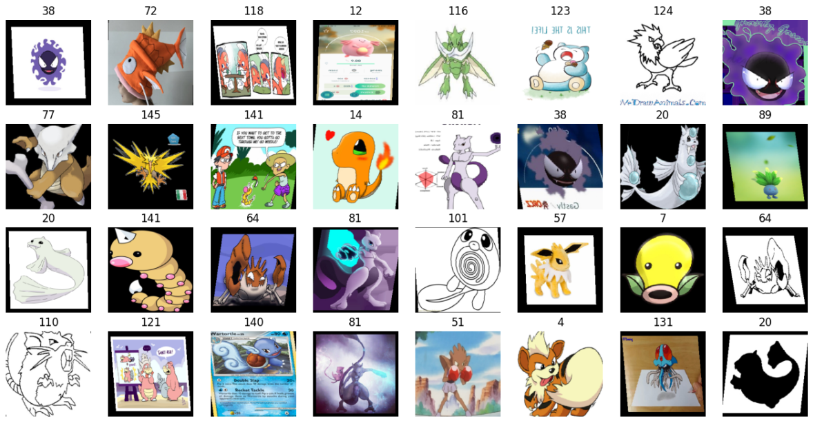
예시 20)
# 배치에서 첫 번째 데이터셋 가져옴
imgs, labels = next(iter(dataloaders['train']))

# 4x8(총 32개)의 서브플롯을 생성하여 이미지를 표시할 공간 만들기
fig, axes = plt.subplots(4, 8, figsize=(16, 8))

# 각 이미지와 라벨을 subplot에 추가
for ax, img, label in zip(axes.flatten(), imgs, labels):
    ax.imshow(img.permute(1, 2, 0))  # PyTorch Tensor 형식(C, H, W)을 (H, W, C)로 변환하여 표시
    ax.set_title(label.item())  # 이미지의 클래스 라벨 표시
    ax.axis('off')  # x, y 축 숨김
--->
예시 21)
image_datasets['train'].classes[21]
-->
Diglett
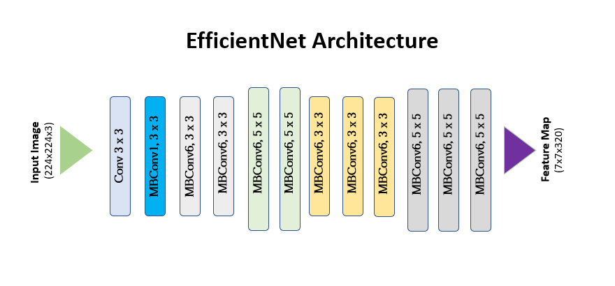
2. EfficientNet
* EfficientNet은 구글에서 개발한 합성곱 신경망(CNN) 모델로, 모델의 크기(depth), 너비(width), 해상도(resolution)를 균형 있게 조정하는 컴파운드 스케일링(compound scaling) 기법을 사용하여 효율성과 성능을 동시에 향상시킨 것이 특징입니다.
* 기존에는 모델의 크기를 단순히 깊게 만들거나(width나 resolution을 개별적으로 확장) 했지만, EfficientNet은 세 가지 요소를 균형 있게 확장하여 연산량을 최적화하면서도 높은 정확도를 유지할 수 있도록 설계되었습니다.
* 특히, EfficientNet-B0을 기본 모델로 하고, B1~B7까지 단계적으로 확장하여 다양한 컴퓨팅 리소스 환경에서 최적의 성능을 낼 수 있도록 제공됩니다.
* EfficientNet은 이미지 분류, 객체 탐지 등 다양한 컴퓨터 비전 작업에서 기존 모델들보다 더 적은 연산량으로도 뛰어난 성능을 보여주며, 실무에서도 널리 활용됩니다.
예시 1)
# EfficientNet B4 모델과 가중치 불러오기
from torchvision.models import efficientnet_b4, EfficientNet_B4_Weights

# 사전 학습된 EfficientNet B4 모델을 로드하고, 가중치를 ImageNet1K에서 가져옴
model = efficientnet_b4(weights=EfficientNet_B4_Weights.IMAGENET1K_V1).to(device)

# 모델 정보 출력
model
--->
# 일부분 출력
Downloading: "https://download.pytorch.org/models/efficientnet_b4_rwightman-23ab8bcd.pth" to /root/.cache/torch/hub/checkpoints/efficientnet_b4_rwightman-23ab8bcd.pth
100%|██████████| 74.5M/74.5M [00:00<00:00, 157MB/s]
EfficientNet(
  (features): Sequential(
    (0): Conv2dNormActivation(
      (0): Conv2d(3, 48, kernel_size=(3, 3), stride=(2, 2), padding=(1, 1), bias=False)
      (1): BatchNorm2d(48, eps=1e-05, momentum=0.1, affine=True, track_running_stats=True)
      (2): SiLU(inplace=True)
    )
    (1): Sequential(
      (0): MBConv(
        (block): Sequential(
          (0): Conv2dNormActivation(
            (0): Conv2d(48, 48, kernel_size=(3, 3), stride=(1, 1), padding=(1, 1), groups=48, bias=False)
            (1): BatchNorm2d(48, eps=1e-05, momentum=0.1, affine=True, track_running_stats=True)
            (2): SiLU(inplace=True)
          )
          (1): SqueezeExcitation(
            (avgpool): AdaptiveAvgPool2d(output_size=1)
            (fc1): Conv2d(48, 12, kernel_size=(1, 1), stride=(1, 1))
            (fc2): Conv2d(12, 48, kernel_size=(1, 1), stride=(1, 1))
            (activation): SiLU(inplace=True)
            (scale_activation): Sigmoid()
          )
          (2): Conv2dNormActivation(
            (0): Conv2d(48, 24, kernel_size=(1, 1), stride=(1, 1), bias=False)
            (1): BatchNorm2d(24, eps=1e-05, momentum=0.1, affine=True, track_running_stats=True)
          )
        )
        (stochastic_depth): StochasticDepth(p=0.0, mode=row)
      )
예시 2)
# 모델의 모든 가중치를 고정 (Feature Extractor로 사용)
for param in model.parameters():
    param.requires_grad = False

# 모델의 분류기(classifier) 부분을 새로운 Fully Connected Layer로 교체
model.classifier = nn.Sequential(
    nn.Linear(1792, 512),  # 기존 특징 벡터 크기(1792) → 512개 뉴런으로 축소
    nn.ReLU(),             # 활성화 함수로 ReLU 사용
    nn.Linear(512, 147)    # 최종 출력 뉴런 개수를 147개로 설정 (147개 클래스 분류)
).to(device)

# 변경된 모델 구조 출력
model
--->
EfficientNet(
  (features): Sequential(
    (0): Conv2dNormActivation(
      (0): Conv2d(3, 48, kernel_size=(3, 3), stride=(2, 2), padding=(1, 1), bias=False)
      (1): BatchNorm2d(48, eps=1e-05, momentum=0.1, affine=True, track_running_stats=True)
      (2): SiLU(inplace=True)
    )
    (1): Sequential(
      (0): MBConv(
        (block): Sequential(
          (0): Conv2dNormActivation(
            (0): Conv2d(48, 48, kernel_size=(3, 3), stride=(1, 1), padding=(1, 1), groups=48, bias=False)
            (1): BatchNorm2d(48, eps=1e-05, momentum=0.1, affine=True, track_running_stats=True)
            (2): SiLU(inplace=True)
          )
          (1): SqueezeExcitation(
            (avgpool): AdaptiveAvgPool2d(output_size=1)
            (fc1): Conv2d(48, 12, kernel_size=(1, 1), stride=(1, 1))
            (fc2): Conv2d(12, 48, kernel_size=(1, 1), stride=(1, 1))
            (activation): SiLU(inplace=True)
            (scale_activation): Sigmoid()
          )
          (2): Conv2dNormActivation(
            (0): Conv2d(48, 24, kernel_size=(1, 1), stride=(1, 1), bias=False)
            (1): BatchNorm2d(24, eps=1e-05, momentum=0.1, affine=True, track_running_stats=True)
          )
예시 3)
## PyTorch의 최적화(Optimizer) module의 import
# import torch.optim as optim

# Adam 옵티마이저를 사용하여 모델의 가중치를 최적화 (학습률: 0.001)
optimizer = optim.Adam(model.parameters(), lr=0.001)

# 학습할 전체 Epoch(반복) 수 설정
epochs = 10
예시 4)
# 전체 Epoch(반복) 동안 학습 및 검증 실행
for epoch in range(epochs):
    # 'train'과 'validation' 단계로 나누어 실행
    for phase in ['train', 'validation']:

        # 훈련 단계에서는 모델을 학습 모드로 설정
        if phase == 'train':
            model.train()
        else:
            model.eval()  # 검증 단계에서는 모델을 평가 모드로 설정

        sum_losses = 0  # 전체 Loss를 저장할 변수
        sum_accs = 0  # 전체 Accuracy(정확도)를 저장할 변수

        # 현재 phase(train 또는 validation)의 데이터 배치를 하나씩 불러옴
        for x_batch, y_batch in dataloaders[phase]:
            x_batch = x_batch.to(device)  # 입력 데이터(batch)를 GPU/CPU로 이동
            y_batch = y_batch.to(device)  # 정답 레이블을 GPU/CPU로 이동

            y_pred = model(x_batch)  # 모델이 예측한 값 계산
            loss = nn.CrossEntropyLoss()(y_pred, y_batch)  # Cross Entropy Loss 계산

            # 훈련 단계에서만 역전파(Backpropagation) 수행하여 가중치 업데이트
            if phase == 'train':
                optimizer.zero_grad()  # 이전 Gradient 초기화
                loss.backward()  # 역전파 수행
                optimizer.step()  # 가중치 업데이트

            sum_losses = sum_losses + loss  # 배치별 손실값 누적

            # 소프트맥스를 사용하여 확률값 변환
            y_prob = nn.Softmax(dim=1)(y_pred)
            y_pred_index = torch.argmax(y_prob, axis=1)  # 가장 높은 확률을 가진 클래스 인덱스 찾기
            acc = (y_batch == y_pred_index).float().sum() / len(y_batch) * 100  # 정확도 계산
            sum_accs = sum_accs + acc  # 배치별 정확도 누적

        # 평균 Loss 및 Accuracy 계산
        avg_loss = sum_losses / len(dataloaders[phase])
        avg_acc = sum_accs / len(dataloaders[phase])

        # 현재 Epoch에 대한 결과 출력
        print(f'{phase:10s}: Epoch {epoch+1:4d}/{epochs} Loss: {avg_loss:.4f} Accuracy: {avg_acc:.2f}%')
        --->
       /usr/local/lib/python3.11/dist-packages/PIL/Image.py:1045: UserWarning: Palette images with Transparency expressed in bytes should be converted to RGBA images
  warnings.warn(
train     : Epoch    1/10 Loss: 3.3476 Accuracy: 29.58%
validation: Epoch    1/10 Loss: 1.4402 Accuracy: 70.03%
train     : Epoch    2/10 Loss: 1.7435 Accuracy: 58.40%
validation: Epoch    2/10 Loss: 0.9472 Accuracy: 77.82%
train     : Epoch    3/10 Loss: 1.3961 Accuracy: 65.13%
validation: Epoch    3/10 Loss: 0.7227 Accuracy: 82.22%
train     : Epoch    4/10 Loss: 1.1739 Accuracy: 70.21%
validation: Epoch    4/10 Loss: 0.6489 Accuracy: 84.41%
train     : Epoch    5/10 Loss: 1.0345 Accuracy: 72.90%
validation: Epoch    5/10 Loss: 0.5870 Accuracy: 85.41%
train     : Epoch    6/10 Loss: 0.9543 Accuracy: 74.34%
validation: Epoch    6/10 Loss: 0.5332 Accuracy: 85.01%
train     : Epoch    7/10 Loss: 0.8413 Accuracy: 77.21%
validation: Epoch    7/10 Loss: 0.5343 Accuracy: 86.30%
train     : Epoch    8/10 Loss: 0.7921 Accuracy: 78.03%
validation: Epoch    8/10 Loss: 0.4924 Accuracy: 87.19%
train     : Epoch    9/10 Loss: 0.7248 Accuracy: 79.49%
validation: Epoch    9/10 Loss: 0.4743 Accuracy: 88.09%
train     : Epoch   10/10 Loss: 0.6839 Accuracy: 80.94%
validation: Epoch   10/10 Loss: 0.5204 Accuracy: 85.60%
예시 5)
import torch  # PyTorch import

# 학습된 모델의 가중치(Weights) 저장
torch.save(model.state_dict(), 'model.pth')
예시 6)
# torchvision에서 사전 학습된 모델 불러옴
from torchvision import models
import torch.nn as nn  # PyTorch 신경망 모듈
import torch  # PyTorch 라이브러리

# EfficientNet-B4 모델을 생성하고 GPU 또는 CPU로 이동
model = models.efficientnet_b4().to(device)

# 기존 분류기(classifier) 부분을 새로운 Fully Connected Layer로 교체
model.classifier = nn.Sequential(
    nn.Linear(1792, 512),  # EfficientNet-B4의 특징 벡터 크기(1792) → 512개 뉴런으로 변환
    nn.ReLU(),             # 활성화 함수로 ReLU 적용
    nn.Linear(512, 147)    # 최종 출력 뉴런 개수를 147개로 설정 (147개 클래스 분류)
).to(device)

# 변경된 모델 구조 출력
model
--->
EfficientNet(
  (features): Sequential(
    (0): Conv2dNormActivation(
      (0): Conv2d(3, 48, kernel_size=(3, 3), stride=(2, 2), padding=(1, 1), bias=False)
      (1): BatchNorm2d(48, eps=1e-05, momentum=0.1, affine=True, track_running_stats=True)
      (2): SiLU(inplace=True)
    )
    (1): Sequential(
      (0): MBConv(
        (block): Sequential(
          (0): Conv2dNormActivation(
            (0): Conv2d(48, 48, kernel_size=(3, 3), stride=(1, 1), padding=(1, 1), groups=48, bias=False)
            (1): BatchNorm2d(48, eps=1e-05, momentum=0.1, affine=True, track_running_stats=True)
            (2): SiLU(inplace=True)
          )
예시 7)
import torch  # PyTorch import

# 저장된 모델 가중치(Weights) 불러오기
model.load_state_dict(torch.load('model.pth'))
-->
<ipython-input-30-fe08fbba245f>:1: FutureWarning: You are using `torch.load` with `weights_only=False` (the current default value), which uses the default pickle module implicitly. It is possible to construct malicious pickle data which will execute arbitrary code during unpickling (See https://github.com/pytorch/pytorch/blob/main/SECURITY.md#untrusted-models for more details). In a future release, the default value for `weights_only` will be flipped to `True`. This limits the functions that could be executed during unpickling. Arbitrary objects will no longer be allowed to be loaded via this mode unless they are explicitly allowlisted by the user via `torch.serialization.add_safe_globals`. We recommend you start setting `weights_only=True` for any use case where you don't have full control of the loaded file. Please open an issue on GitHub for any issues related to this experimental feature.
  model.load_state_dict(torch.load('model.pth'))
<All keys matched successfully>
예시 8)
model.eval() # 모델을 평가 모드
--->
EfficientNet(
  (features): Sequential(
    (0): Conv2dNormActivation(
      (0): Conv2d(3, 48, kernel_size=(3, 3), stride=(2, 2), padding=(1, 1), bias=False)
      (1): BatchNorm2d(48, eps=1e-05, momentum=0.1, affine=True, track_running_stats=True)
      (2): SiLU(inplace=True)
    )
    (1): Sequential(
      (0): MBConv(
        (block): Sequential(
          (0): Conv2dNormActivation(
            (0): Conv2d(48, 48, kernel_size=(3, 3), stride=(1, 1), padding=(1, 1), groups=48, bias=False)
            (1): BatchNorm2d(48, eps=1e-05, momentum=0.1, affine=True, track_running_stats=True)
            (2): SiLU(inplace=True)
          )
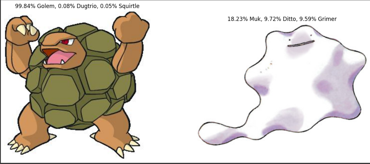
샘플로 포켓몬스터 그림을 첨부하여 몇퍼센트에 가까운지 알아보자
예시 9)
from PIL import Image  # 이미지 파일을 다루기 위한 PIL(Pillow) import
import matplotlib.pyplot as plt  # 이미지 시각화를 위한 Matplotlib import

# 두 개의 이미지 파일을 열기 (PIL Image 객체로 변환)
img1 = Image.open('/content/test/mon1.jpg')
img2 = Image.open('/content/test/mon2.jpg')

# 1행 2열의 서브플롯(subplot) 생성 (이미지를 나란히 배치)
fig, axes = plt.subplots(1, 2, figsize=(12, 6))

# 첫 번째 이미지 표시
axes[0].imshow(img1)  # img1을 첫 번째 서브플롯(왼쪽)에 출력
axes[0].axis('off')  # x, y 축 제거 (이미지만 보이도록 설정)

# 두 번째 이미지 표시
axes[1].imshow(img2)  # img2를 두 번째 서브플롯(오른쪽)에 출력
axes[1].axis('off')  # x, y 축 제거

# 최종적으로 화면에 표시
plt.show()
--->

예시 10)
# 'validation' 데이터 변환을 적용하여 이미지를 모델 입력 형태로 변환
img1_input = data_transforms['validation'](img1)
img2_input = data_transforms['validation'](img2)

# 변환된 이미지의 텐서(shape) 출력
print(img1_input.shape)
print(img2_input.shape)
-->
torch.Size([3, 224, 224])
torch.Size([3, 224, 224])
예시 11)
# 두 개의 변환된 이미지 텐서를 하나의 배치(batch)로 쌓음
test_batch = torch.stack([img1_input, img2_input])

# 배치를 GPU 또는 CPU로 이동
test_batch = test_batch.to(device)

# 배치의 텐서(shape) 출력
test_batch.shape
-->
torch.Size([2, 3, 224, 224])
예시 12)
# 모델에 배치(batch) 데이터를 입력하여 예측 수행
y_pred = model(test_batch)

# 예측 결과 출력
y_pred
--->
tensor([[-12.6083, -21.3744, -14.6089, -18.9894,  -9.2162, -25.5719, -18.1158,
         -18.1595,  -9.2986,  -7.8870, -19.3475,  -9.7119, -19.0499, -20.0923,
          -7.7194, -13.7215, -21.2366, -17.0407, -18.4799,  -9.6722, -19.7328,
          -6.0974, -14.9443, -17.5417, -17.4903, -28.3349, -17.2331, -21.8986,
          -9.8076,  -1.9439, -14.4411,  -9.4540, -16.8286, -23.1351, -15.4615,
         -14.8586, -13.8246, -14.4821, -17.2461, -16.0954,  -5.2603, -15.1820,
         -19.4468, -21.6349, -11.5953,   5.1906,  -6.6062,  -9.6074,  -8.0349,
         -16.7220, -23.5732, -12.2040, -10.6822, -18.5408,  -9.6178, -17.5184,
         -14.4301, -16.3119,  -9.1690,  -9.2525, -12.2039, -13.4944,  -9.7138,
          -5.5315, -14.6240, -13.0792, -12.6810, -17.9201, -12.2607, -15.2416,
         -10.4390,  -9.0373, -15.3671, -12.4228, -17.0317, -23.0906, -12.3740,
         -15.9740, -14.4779, -12.7976, -18.9449, -19.3660, -20.0671, -14.7934,
          -9.3139,  -6.5523,  -8.1325, -17.5784, -16.0908, -16.7520, -11.4507,
         -15.5151, -12.5210,  -9.2817, -12.1415, -22.3224, -15.4137, -10.8905,
         -11.8193, -11.4487, -14.6279, -21.3541, -18.1350, -15.0847, -18.1212,
         -13.2224,  -9.1428,  -7.6771, -13.1498, -19.5129, -15.2817, -11.8404,
         -13.4362,  -9.7359,  -3.7391, -11.6367, -17.9746, -19.2129, -22.2101,
         -13.2687, -13.5819, -12.4057, -17.9905, -13.3784, -16.6720,  -2.3239,
         -15.5097, -11.8812, -16.3371, -12.3870, -18.1878, -22.4088, -18.8230,
         -22.2840, -17.3485, -10.5694, -18.7479, -17.2813, -24.0459, -15.8299,
         -12.5965, -12.6951, -22.9748, -14.3797, -18.8467, -25.6792, -23.9534],
        [ -4.5352,  -4.6305,  -6.3427,  -5.7689,  -5.9831,  -8.9581,  -9.4569,
          -6.3650,  -9.7458,  -2.7666,  -8.8823,  -4.8978,  -7.5884,  -7.8470,
          -6.3085,  -5.6841,  -7.6022,  -8.0128,  -2.6733,  -2.9422,  -5.4681,
          -7.4060,  -2.1399, -10.1120,  -7.8582,  -9.6586,  -9.2353,  -6.6509,
          -5.0378,  -6.4197,  -8.2359,  -4.1318, -10.4172,  -8.5780,  -8.8782,
          -7.7843,  -3.8424,  -6.4754,  -6.0726,  -5.7024,  -4.8748,  -9.0513,
          -6.0560,  -5.5863,  -4.9029,  -5.2463,  -5.7434,  -2.1536,  -7.6235,
          -8.1694,  -5.2724,  -5.9154,  -6.1144,  -8.1770,  -4.2230,  -9.1482,
          -8.2747,  -6.5940,  -6.0359,  -6.1191,  -4.6785,  -6.7625,  -5.8156,
          -5.3079,  -6.3794,  -5.4986,  -6.7628,  -5.3734,  -5.5869,  -5.8807,
          -6.1640,  -5.1561,  -7.6601,  -8.8029,  -8.3434, -11.2458,  -4.3309,
          -3.5602,  -9.3940,  -2.5742,  -6.4681,  -3.9571,  -5.4873,  -1.5110,
          -5.5824,  -7.7901,  -6.1590,  -3.8671,  -4.8917,  -8.5199,  -7.2359,
          -7.6691,  -4.5776, -10.4461,  -7.5903,  -7.4531,  -7.4212,  -6.6941,
          -4.8807,  -7.1326,  -7.6295,  -8.5439,  -7.2000,  -7.3996,  -5.1531,
          -8.5522,  -5.5073,  -3.8654, -10.0965,  -3.4378,  -8.0403,  -7.4947,
          -8.3922,  -4.2595,  -6.1589,  -6.4925,  -4.2492,  -6.5954,  -8.0804,
          -7.1474,  -6.7441,  -8.7220,  -7.4942,  -7.0149,  -3.5186,  -6.1205,
          -9.3374,  -6.1917,  -9.4752,  -6.4113,  -7.5763,  -6.8836,  -6.1617,
          -6.2137,  -8.7036,  -7.2165,  -5.9842,  -6.0011, -10.5479,  -7.1116,
          -7.3648,  -6.1278,  -6.8035,  -6.1220,  -9.8611,  -9.3416,  -6.9286]],
       device='cuda:0', grad_fn=<AddmmBackward0>)
예시 13)
import torch.nn as nn

# y_pred는 신경망의 출력(로짓, logits)으로, 아직 확률값이 아닌 원시 점수 형태
# 예를 들어, y_pred가 (batch_size, num_classes) 형태의 텐서라고 가정

y_prob = nn.Softmax(1)(y_pred)  # 소프트맥스(Softmax) 함수 적용 (dim=1, 즉 클래스 차원 기준)

# Softmax는 입력값을 0~1 사이의 확률 값으로 변환하며, 각 샘플(batch)별로 클래스 확률의 총합이 1이 되도록 만듭니다.
# 예를 들어, y_pred가 (2, 3) 크기의 텐서라면, 각 행(row)에 대해 softmax를 적용하여 클래스별 확률을 구함

y_prob  # 이제 y_prob에는 각 클래스에 대한 확률값이 저장
예시 14)
import torch

# 예제 y_prob (softmax를 적용한 확률값)
y_prob = torch.tensor([[0.1, 0.6, 0.3],
                        [0.2, 0.5, 0.3]])

# top-k (상위 k개) 확률값과 해당 인덱스를 가져옴
probs, idx = torch.topk(y_prob, k=3)

print(probs)  # 상위 3개의 확률값
print(idx)    # 해당 확률값의 클래스 인덱스
-->
tensor([[9.9843e-01, 7.9589e-04, 5.4424e-04],
        [1.8232e-01, 9.7216e-02, 9.5893e-02]], device='cuda:0',
       grad_fn=<TopkBackward0>)
tensor([[ 45,  29, 125],
        [ 83,  22,  47]], device='cuda:0')
예시 15)
import matplotlib.pyplot as plt

# 서브플롯 생성 (1행 2열), 전체 크기는 (15, 6)
fig, axes = plt.subplots(1, 2, figsize=(15, 6))

# 첫 번째 이미지에 대한 예측 결과를 제목으로 설정
axes[0].set_title('{:.2f}% {}, {:.2f}% {}, {:.2f}% {}'.format(
    probs[0, 0] * 100,  # 첫 번째로 높은 확률 (% 변환)
    image_datasets['validation'].classes[idx[0, 0]],  # 해당 클래스 이름
    probs[0, 1] * 100,
    image_datasets['validation'].classes[idx[0, 1]],
    probs[0, 2] * 100,
    image_datasets['validation'].classes[idx[0, 2]],
))
axes[0].imshow(img1)  # 첫 번째 이미지 표시
axes[0].axis('off')  # 축 눈금 제거

# 두 번째 이미지에 대한 예측 결과를 제목으로 설정
axes[1].set_title('{:.2f}% {}, {:.2f}% {}, {:.2f}% {}'.format(
    probs[1, 0] * 100,
    image_datasets['validation'].classes[idx[1, 0]],
    probs[1, 1] * 100,
    image_datasets['validation'].classes[idx[1, 1]],
    probs[1, 2] * 100,
    image_datasets['validation'].classes[idx[1, 2]],
))
axes[1].imshow(img2)  # 두 번째 이미지 표시
axes[1].axis('off')  # 축 눈금 제거

plt.show()  # 그래프 출력
--->
자신의 닮은 꼴 캐릭터 찾기
예시 1)
mypic = Image.open('/content/test/mypic.jpg')
plt.imshow(mypic)
plt.axis('off')
예시 2)
mypic_input = data_transforms['validation'](mypic)  # 이미지 변환 적용
print(mypic_input.shape)  # 변환된 이미지의 텐서 형태 출력

mypic_input = mypic_input.unsqueeze(0).to(device)  # 배치 차원 추가 및 GPU/CPU로 이동
print(mypic_input.shape)  # 최종 입력 텐서의 형태 출력
예시 3)
y_pred = model(mypic_input)  # 모델에 입력을 전달하여 예측 수행
y_pred  # 모델의 출력값 (로짓, logits)
예시 4)
import torch.nn as nn

# Softmax를 적용하여 확률값 변환
y_prob = nn.Softmax(1)(y_pred)
y_prob  # 각 클래스에 대한 확률값 출력
예시 5)
import torch

# 가장 확률이 높은 상위 3개 클래스와 해당 확률값을 가져옴
probs, idx = torch.topk(y_prob, k=3)

print(probs)  # 상위 3개 클래스의 확률값
print(idx)    # 상위 3개 클래스의 인덱스
예시 6)
import matplotlib.pyplot as plt

# 그래프 제목을 설정하여 상위 3개 클래스의 예측 결과 표시
plt.title('{:.2f}% {}, {:.2f}% {}, {:.2f}% {}'.format(
    probs[0, 0] * 100,  # 가장 높은 확률 클래스의 확률(% 변환)
    image_datasets['validation'].classes[idx[0, 0]],  # 가장 높은 확률 클래스 이름
    probs[0, 1] * 100,
    image_datasets['validation'].classes[idx[0, 1]],
    probs[0, 2] * 100,
    image_datasets['validation'].classes[idx[0, 2]],
))

# 예측할 이미지 표시
plt.imshow(mypic)
plt.axis('off')  # 축 눈금 제거
plt.show() # 이미지 출력'컴퓨터 비전' 카테고리의 다른 글
| OCR (6) | 2025.03.06 |
|---|---|
| 4-(2). OpenCV (0) | 2025.03.05 |
| 4. OpenCV (0) | 2025.03.05 |
| 2. Classification (0) | 2025.02.28 |
| 1. 컴퓨터 비전(Computer Vision) (4) | 2025.02.28 |